Forecasting Footfall on Hampstead Heath

Description

Using a mobile phone derived human locaiton dataset, random forest model & interactive R Shiny dashboard to forecast footfall on Hampstead Heath under specified time & wather conditions.

The Problem Space & Motivations for Tackling it

I chose this topic because I wanted to combine my passion for the outdoors with data science, and mobile phone location data is increasingly central to business decisions and planning, so I was excited to get some hands on experience with it.

Whilst my dissertatioin was an extensive exploratory analysis, and an in depth look at the merits of big data versus other more traditional research methods (namely in person observations), I wanted to push the potentials of the dataset further, to explore how more complex modelling might be applied, to enable the dataset to serve as a tool that could aid future planning/ logistics/ resource allocation etc.

The Data

Data for this project was compiled from 3 key sources joined and cleaned in R [(see code for this workflow here)](link/to/code:

1. Footfall Data

The human location data for this project was kindly provided by WhereData

• Data was shared for the London boroughs of Camden and Barnet, covering July - December 2023 (providing a 6-month test case through which to explore the tool’s potential, with clear value if this were to be extended to a full year and beyond)
• Footfall estimates are aggregated to hourly counts, at the spatial resolution of Uber’s H3 Grid Level 10
• The data is sourced from anonymised, consented-to app location signals, collected from a panel that is representative of the UK population

2. Weather Data

Historical hourly weather records were downloaded in batches from [VisualCrossing.com]

• The dataset contained 10+ variables, but only temperature and precipitation were included in the final model - following extensive exploration

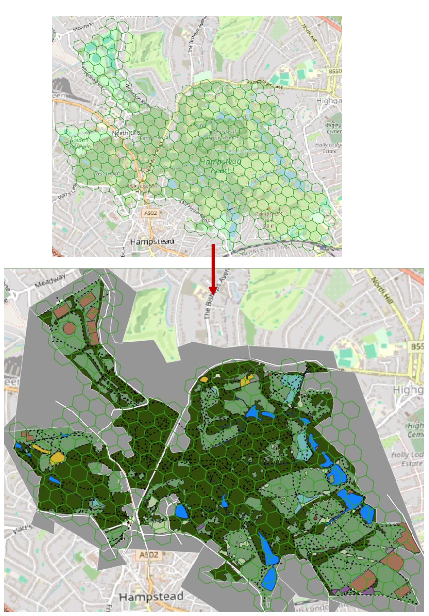
3. Spatial Features

The physical features within each hexagon cell were quantified using QGIS. OSM was traced to vectorise features, before forming cell overlap calculations to quantify them according to the type of feature:

• Point features (benches, cafes, attractions) → Point in polygon calc
• Line feature (paths, boundaries…) → Length in polygon calc
• Polygon features → Area in polygon overlap calc

Methodology

Overview: Following extensive EDA which formed the bulk of the dissertation, Random Forest model was used to make predictions for the R Shiny dashboard.

Exploratory Analysis

You can view the full code here

(plots taken from dissertation)

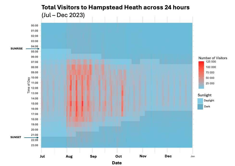
• Clear seasonal and weekly patterns emerged from the data: a strong upturn in visits at the turn of August & consistent weekend daytime peaks - Interesting spike on the second weekend of October, and absence of weekend uplift mid-November

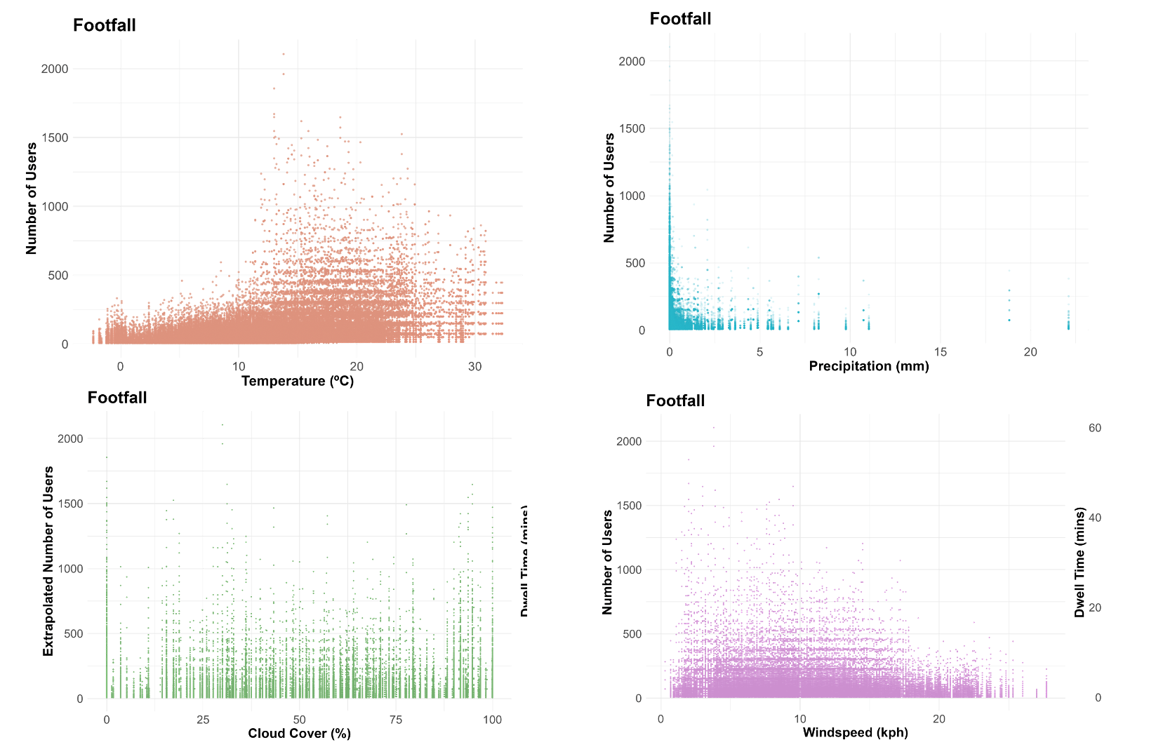
• Temperature and Precipitation exhibit the strongest potential relationship with footfall
• Visits taper off less dramatically with increased windspeeds, whilst cloud cover doesn’t appear to exhibit a relationship

In my dissertation, I also applied a hierarchical clustering algorithm to the data (Ward’s Agglomerative Linkage method). From this, it was clear that areas with similar spatial features exhibited similar visitation regimes that were distinct between identified clusters - therefore it was obvious that spatial features needed to be included in any good predictive model.

Devising a Predictive Model

You can view the full code here

→ Random Forest model was selected for this task due to its ability to capture complex, non-linear relationships.

Tracking Experiments

Due to technical restraints with setting up virtual environments on the remote desktop I was working on (required for sufficient computing power to handle the dataset), this ML model was built using R (my first and likely last experience doing so: though its possible in R, I found that Python syntax definitely lends itself more intuitively to ML!)

→ step 1 was to write a tracking function that emulated function of Python’s MLflow

Approach to modelling

→ I took a random 80/20 train test split. Whilst I considered stratification (which can be useful particularly on smaller or highly imbalanced datasets) in this case (given the hundereds of thousands of observations) it risked over-engineering the split and potentially artificially inflating performance. A random split provided a more robust assssment of generalisability.

1. Firstly established a baseline accuracy by selecting the most appropriate features to include in the model - aiming to balance accuracy with minimal complexity. I ran initial models that isolated 3 key types of predictor varaibles in turn - examining feature importance each time: - Time variables (month, day of week, hour) - Weather variables (precipitation, temperature) - Spatial variables (presence of benches, grass, woodland, water, paths, sports facilities, attractions, cafes, distance from park perimeter)

Without including a combination of variables from all 3 variable types, initial runs performed poorly - successfully capturing just 16% of variation in the data (including temporal variables alone), and 66% for spatial variables only - which is slightly better but still equates to a RMSE of 300 (significant considering that cells pretty rarely exceed 305 visitors in an hour)

2. Initially I included all cells that covered the Heath in any amount - to see how well the model might be able to account for ‘noise’ external to the park, with a variable capturing the % of the cell’s area that was non park, and the length of any road passing through it. With this noise in the data, I struggled to improve predictive accuracy beyond 70% - Before the train-test split occured, I went back and removed any cell containing road, and any cell containing > 10% land that was non park. - Performance immediately jumped to 82% from here (RMSE down to 22).

If I further quantified the spatial features external to the park this likely wouldn’t be a neccessary step. If we were trying to predict footfall for urban areas a whole though, it would also require careful consideration of another set of predictor variables (such as school dropoff times, type of road, classified as residential etc, taking account of trainlines). Given that the predictors in this dataset were devised specifically with parks in mind (and based on my own observations of movement across the space), it makes sense that these cells introduced noise, and predictions drastically improved on their removal.

3. The final step was to tune hyperparameters. I experimented with: - Number of trees: - Minimum node size: - Number of features considered at each split

The Final Dashboard.